Statistical Analyses
The pipeline for detecting vote dilution, highlighted in the eiCompare page, requires the application of several analysis techniques such as ecological inference (EI), Bayesian Improved Surname Geocoding (BISG), and a performance analysis. In this section, we detail these analyses, their components, and limitations. Each of these analyses are incorporated into eiCompare to facilitate detection of vote dilution across a broad array of datasets.
Ecological Inference
As stated in the Motivation page, voting rights litigation relies on the Gingles Test, which requires the following conditions to be satisfied for a Voting Rights Act violation:
- The group of minority voters is sufficiently large and geographically compact.
- Minority voters are politically cohesive in supporting their candidate of choice
- The majority votes in a bloc to usually defeat the minority’s preferred candidate.
The datasets we have access to, as described in Methods, provide us information about who voted (from the voter file) and which candidates received votes (from the election results). Knowing these totals isn’t good enough to meet the requirements of the Gingles test - we actually need to know which candidates voters supported in order to determine whether majority voters and minority voters were cohesive blocks supporting different candidates (criteria 2 and 3). By law, the specific candidates chosen by a voter are secret to ensure the voter’s privacy. Thus, we need to infer these quantities from the data.
At first glance, this may seem impossible. For example, consider a toy election with White and Black voters choosing between Candidates A and B (Figure 1, left). We might know the marginal data – the totals for each row and column, as shown – but we don’t know the individual entries in the table (Figure 1: question marks). The voters could be split into any number of assortments across the four individual blocks that satisfy the requirement of adding up to the marginals. How do we choose the most reasonable vote allocation?
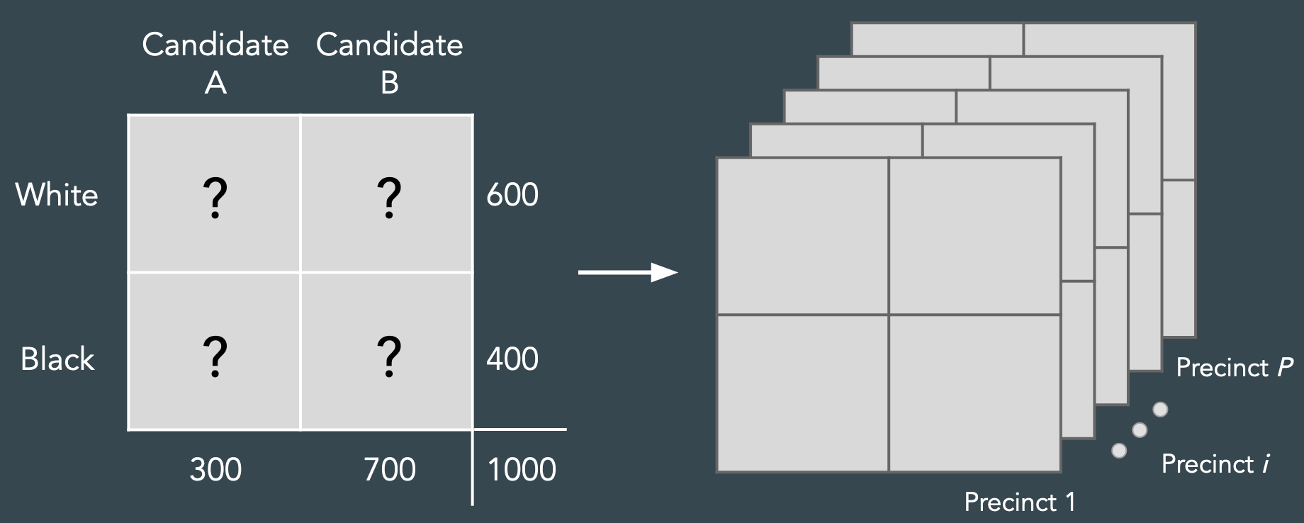
Figure 2: The ecological inference problem.
A closer inspection reveals we have more information that we can tap into. Election data typically consists of voter turnout and results across precincts, which are smaller geographic units in the electoral district. Thus, instead of having one table with known marginals, we actually have many tables (one for each precinct: see Figure 1, right). If we reasonably assume that racial groups don’t vote too differently across precincts, we can leverage the statistical regularities in voting patterns across the tables to infer what fraction of voters support different candidates, across racial groups. This is the ecological inference (EI) problem: using patterns in ecological units (in this case, precincts) to infer (aggregated) individual-level (voters) behavior.
There are a variety of approaches to solve the ecological inference problem.
These approaches generally assume an underlying statistical model describing
voting patterns that can be fit to the data. Currently, two approaches are
predominantly used in voting rights litigation: King’s iterative EI (King et
al., 1997) and rows by columns (RxC) method (Rosen et al., 2001). Both
approaches have their pros and cons. The eiCompare package helps facilitate
comparisons between these approaches.
See the EI vignette for details on how to use eiCompare to apply EI to voter
data.
Bayesian Improved Surname Geocoding
To proceed with ecological inference, we need accurate counts of the turnout by racial group (Figure 5: row marginals). Ultimately, this requires knowledge of each voter’s race, which is not always provided on the voter file. In the cases where we don’t have access to each voter’s race, we need to estimate it from the data. We use an approach called Bayesian Improved Surname Geocoding (BISG) to obtain probabilistic estimates of each voter’s race in a voter file, which can then be used to estimate turnout by race across precinct.
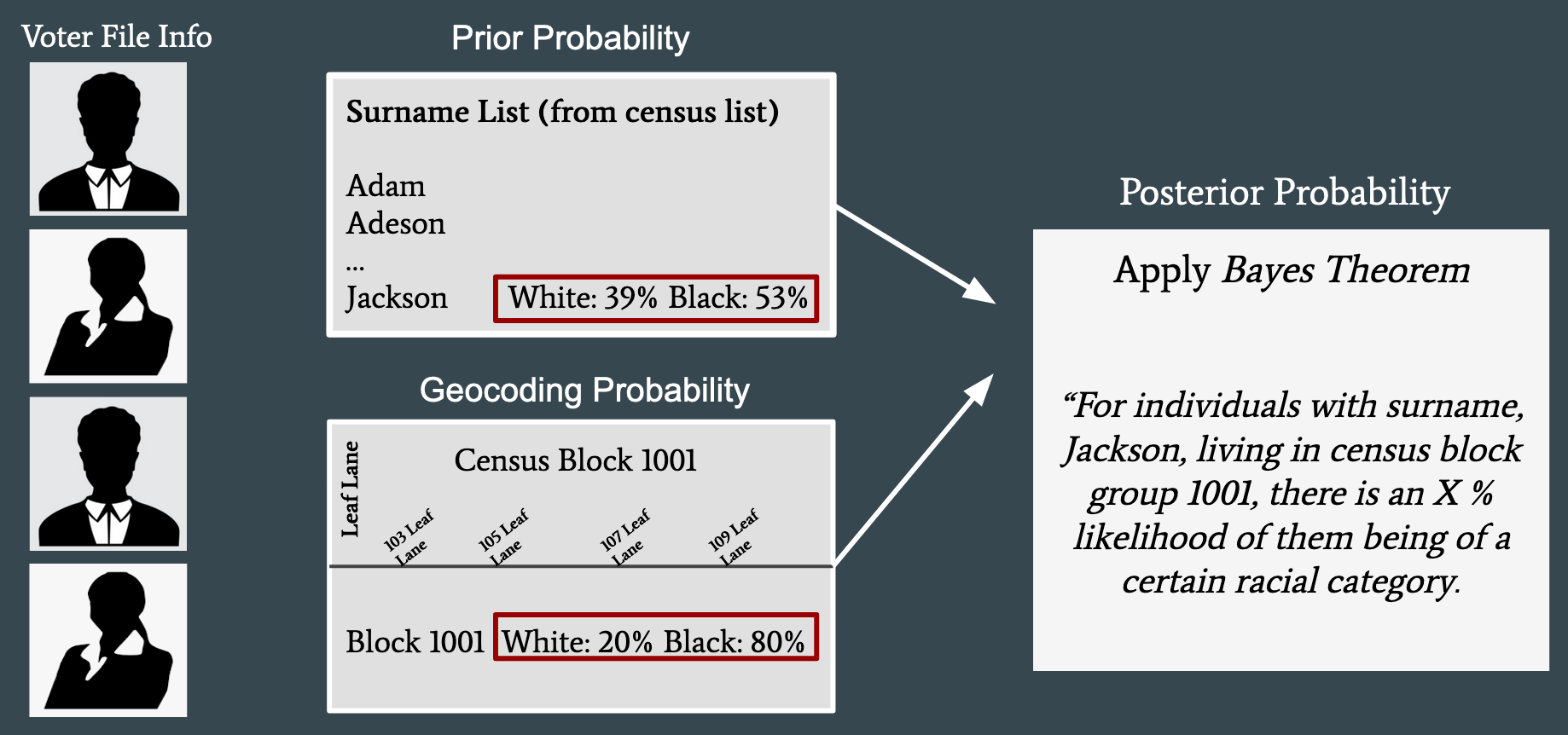
Figure 2: BISG leverages surnames and location to obtain a probabilistic estimate of race.
BISG relies on the observation that both a person’s surname and location are informative about their race (Elliott et al., 2009). It crucially relies on the Census Bureau’s comprehensive database of surnames and tabulation of racial groups in geographic blocks across the United States. To apply BISG, we first assume that a person’s surname provides prior knowledge of what their race might be (e.g., a person with a surname of “Jackson” has a 53% chance of being black: Figure 2). Next, we use that voter’s location to“update” the probability to a posterior probability of race using Bayes’ Theorem. For example, if the person with the surname “Jackson” lives in a Census block with self-reported race of constituents being predominantly black (in 2010), that greatly increases the probability that they are black.
In practice, we utilize the package WRU (“Who Are You”) provided by Imai and Khanna (2016) to calculate the BISG. This package also allows updating the posterior probability using knowledge of a voter’s sex, age, and party affiliation, though in practice these latter features may have limited impact on the posterior probabilities.
See the BISG vignette for more details.
Performance Analyses
The ultimate outcome from voting rights litigation is to produce a districting map that allows adequate representation for minority groups, prompting the need for a new districting map. Thus, we need to assess whether the new districting map provides sufficient representation for minority groups. To do so, we can look at past elections, and observe how candidates would perform if the proposed map was used at the time (how it would “perform”) of the election. This is the basis of a performance analysis.
Importantly, a performance analysis should be performed with the voter turnout data rather than the registered voter data or tabulations of eligible voters. The voter turnout data reflects who actually voted in the election, rather than who might have voted.
See the performance analysis vignette for more
details on how to use eiCompare to run a performance analysis.
References
-
Elliott, M. N., Morrison, P. A., Fremont, A., McCaffrey, D. F., Pantoja, P., & Lurie, N. (2009). Using the Census Bureau’s surname list to improve estimates of race/ethnicity and associated disparities. Health Services and Outcomes Research Methodology, 9(2), 69.
-
King, G. (1997). A solution to the ecological inference problem: reconstructing individual behavior from aggregate data. Princeton: Princeton University Press.
-
Imai, K., & Khanna, K. (2016). Improving ecological inference by predicting individual ethnicity from voter registration records. Political Analysis, 263-272.
-
Rosen, O., Jiang, W., King, G., Tanner, M.A. (2001). Bayesian and frequentist inference for ecological inference: the R x C case. Statistica Neerlandica, 55, 2, p. 134-156.