eiCompare: Ecological Inference
This vignette illustrates how we can use the Ecological Inference (EI)
tools within eiCompare to learn about the voting behavior of different
groups of voters.
The ecological inference problem
Ecological Inference involves estimating the voting behaviors of different groups of voters using only data about election results and the number of people from each group that turned out to vote. Elections in the United States, and much of the rest of the world, use secret ballots that ensure confidentiality for every voter. Voter confidentiality is important for a functioning democracy, but it presents a problem for those who want to learn about voter behavior. We cannot directly measure how people vote in an election. Intead, we have to make inferences about how they might have voted using election results and information about voter turnout. We often end up with datasets like the following, which contains aggregate election results and turnout information for each election precinct in Gwinnett County, Georgia:
suppressPackageStartupMessages({
  library(eiCompare)
  library(dplyr)
})

data("gwinnett")
head(gwinnett)
#>   precinct turnout kemp abrams metz white black hispanic other
#> 1      001    3718 1835   1842   41  1862  1247      211   522
#> 2      002    2251  434   1805   12   455  1447       68   268
#> 3      003    2721 1156   1532   33  1147   850      220   399
#> 4      004     875  402    456   17   522   188       36   134
#> 5      005    1765  963    783   19  1004   477       36   222
#> 6      006    2116  841   1248   27   915   520      255   394
This dataset contains the following columns:
precinct- This uniquely identifies each precinct in the county.turnout- The total number of voters who cast ballots on election daykemp,abrams,metz- These count the number of votes cast for each candidate.white,black,hispanic,other- These count the number of voters who self-reported as each race group.
Election results by precinct are generally accessible online from election administrators. Measuring the turnout of different racial/ethnic groups, however, can present more of a challenge. Luckily, the state of Georgia requires voters to self-report their race when they register. This means anyone can tabulate the number of voters self-reporting with each group in each precinct, provided they gain access to a voter file. That’s exactly what we’ve done here. To learn more about how to estimate voters’ race based only on their name and address, see the tutorials on Geocoding voter files and Bayesian Improved Surname Geocoding
We know the number of votes cast for each candidate and by each racial/ethnic group. From this data, we want to learn whether voters from different ethnic groups prefer different candidates.
Preparing the data
First, we need to clean and prepare the data. eiCompare contains functions to
streamline data preparation and prevent common errors that emerge during this
process.
First, let’s set up our column vectors. Most eiCompare functions for ecological inference require these as parameters.
cands <- c("kemp", "abrams", "metz")
races <- c("white", "black", "hispanic", "other")
total <- "turnout"
id <- "precinct"
We start by dealing with all the missing values in the our dataset. For this, we can use the function resolve_missing_vals() from the eiCompare package. This function checks looks for missing values in they important columns of the dataframe. It currently has two options for handling missing values.
na_action = "DROP": The function will drop any row with a missing value.na_action = "MEAN": The function will replace missing values in these columns with their respective column’s mean value.
gwinnett <- resolve_missing_vals(
  data = gwinnett,
  cand_cols = cands,
  race_cols = races,
  totals_col = total,
  na_action = "DROP"
)
#> No missing values in key columns. Returning original dataframe...
Looks like this dataset doesn’t contain any missing values. We can proceed to the next step. Next, we use dedupe_precincts() to check that the data does not contain anyduplicate precincts.
gwinnett <- dedupe_precincts(
  data = gwinnett,
  id_cols = id
)
#> Warning in dedupe_precincts(data = gwinnett, id_cols = id): Precincts appear duplicated. Returning boolean column identifying
#> duplicates...
We got a warning indicating that some rows of the data do appear to belong to the same precinct. When dedupe_precincts() identifies duplicates that it does not know how to resolve, the function returns a column called duplicate that highlights the duplicated rows. This helps us investigate the duplicates and try to figure out where they came from. Let’s take a look at these now.
gwinnett %>%
  filter(duplicate)
#>   precinct turnout kemp abrams metz white black hispanic other
#> 1      035    1658  803    835   20  1100   525       81   362
#> 2      035     368  159    207    2  1100   525       81   362
#>   duplicate
#> 1      TRUE
#> 2      TRUE
Here we see that precinct 035 appears to have entered the data twice. This anomaly has at least two possible explanations:
-
For most elections, precincts report their own results and data entry is often done by hand. This can lead to small mistakes like a precincts’ vote tallies being split over two rows.
-
Election results databases typically contain the resutls of many elections that took place in different jurisdictions and at different times. When extracting the results of a particular election, an easy mistake is to accidentally extract some results from other elections, leading to repeated precinct IDs.
In this case, we have confidence that this duplicate has emerged through an error in precinct reporting. We can combine the two columns using this code:
missing_inds <- which(gwinnett$duplicate)
columns_to_add <- c(total, cands)
gwinnett[missing_inds[1], columns_to_add] <-
  gwinnett[missing_inds[1], columns_to_add] +
  gwinnett[missing_inds[2], columns_to_add]
gwinnett <- gwinnett[-missing_inds[2], ]
gwinnett[missing_inds[1], ]
#>    precinct turnout kemp abrams metz white black hispanic other
#> 35      035    2026  962   1042   22  1100   525       81   362
#>    duplicate
#> 35      TRUE
Now we see the vote totals from the previous two columns have been summed together in this new row. We can double check that this eliminated all duplicates be running dedupe_precincts() again.
gwinnett <- dedupe_precincts(
  data = gwinnett,
  id_cols = id
)
#> Data does not contain duplicates. Proceed...
Now we’re sure that our dataset does not contain any missing values or duplicated precincts. We can proceed with standardizing the data. To execute ecological inference cleanly, we need to make sure to represent our data in proportions that sum to one. Not doing this can cause the EI functions to break or behave unexpectedly. For this, we can use stdize_votes_all().
gwinnett_ei <- stdize_votes_all(
  data = gwinnett,
  cand_cols = cands,
  race_cols = races,
  totals_col = total
)
#> Using provided totals...
#> Standardizing candidate columns...
#> All columns sum correctly. Computing proportions...
#> Standardizing race columns...
#> Vote sums deviate from totals.
#> Deviations are minor. Restandardizing vote columns...
head(gwinnett_ei)
#>     kemp abrams     metz  white  black hispanic  other turnout
#> 1 0.4935 0.4954 0.011027 0.4846 0.3246  0.05492 0.1359    3842
#> 2 0.1928 0.8019 0.005331 0.2033 0.6466  0.03038 0.1197    2238
#> 3 0.4248 0.5630 0.012128 0.4385 0.3249  0.08410 0.1525    2616
#> 4 0.4594 0.5211 0.019429 0.5932 0.2136  0.04091 0.1523     880
#> 5 0.5456 0.4436 0.010765 0.5773 0.2743  0.02070 0.1277    1739
#> 6 0.3974 0.5898 0.012760 0.4391 0.2495  0.12236 0.1891    2084
This function has produced a new dataframe where each column is a proportion. We can check that for each row, the candidate columns sum to one and the race columns sum to one using the following code.
cand_sums <- sum_over_cols(data = gwinnett_ei, cols = cands)
race_sums <- sum_over_cols(data = gwinnett_ei, cols = races)
table(cand_sums, race_sums)
#>          race_sums
#> cand_sums   1
#>         1 156
Here we see that, for each row in the dataset, the sum of the race columns equals one, and the sum of the candidate columns also equals one. We always need to satisfy this condition before running the EI functions.
We now have a new dataframe without missing values, with no duplicated precincts, and with standardized candidate and racial vote proportion colums. We can begin conducting ecological inference.
Descriptive Analysis
Now that we’ve cleaned and prepared the data, we’re ready to begin analyzing it. Before running ecological inference, it’s useful to conduct some simple descriptive analyses. First, let’s plot the precinct-level bivariate relationships between all the different combinations of racial and candidate turnout proportions.
plot_bivariate(
  data = gwinnett_ei,
  cand_cols = cands,
  race_cols = races
)
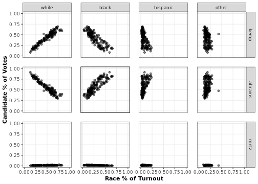
The plot_bivariate() function returns a ggplot2 object plotting the relationships between each candidate’s precinct-level vote share and the precinct-level turnout share of each race group. These plots can tell us a lot about what to expect from the EI analysese to come. In particular, we can observe the following two trends.
-
We observe what looks like racially polarized voting in the top left corner of this figure. The panel in the upper left corner shows that as the proportion of white voters in a precinct rises, so does the proportion of votes for Brian Kemp. The plot just below shows that the opposite is true for Stacey Abrams. Meanwhile, the second column reveals the opposite pattern for black voters. This is a sign that racially polarized voting might be going on in this election. We can use EI to back this up statistically.
-
The bottom row shows that Jim Metz received very few votes across precincts. Because there is so little variation in levels of vote share for this candidate, our EI estimates probably will not detect racially polarized voting for this candidate. We can expect similarly from the ‘hispanic’ and ‘other’ race categories, since few districts have very high proportions of these groups.
We can also get the simple correlation coefficients for each bivariate relationship using the race_cand_cors() function.
race_cand_cors(
  data = gwinnett_ei,
  cand_cols = cands,
  race_cols = races
)
#>          white   black hispanic   other
#> kemp    0.9593 -0.8538  -0.5793 -0.3089
#> abrams -0.9618  0.8602   0.5751  0.3028
#> metz    0.5622 -0.6538  -0.1286  0.0726
For black, white and hispanic voters we observe strong correlations between racial composition and the share of votes going to each candidate. This provides further a indication that ecological inference may reveal racially polarized voting.
These basic descriptive checks help us understand our data and give us a sense of what to expect in our final results. Next, we turn to executing and comparing the different EI techniques.
Ecological Inference
eiCompare enables users to analyze and compare the two dominant EI methods, Iterative EI and RxC EI. For more information about these techniques, see the technical details page of our website.
We can run both methods with their respective functions. They take some time to run because they both compute point estimates by sampling from a distribution.
ei_results_iter <- ei_iter(
  data = gwinnett_ei,
  cand_cols = cands,
  race_cols = races,
  totals_col = total,
  name = "Iter"
)

summary(ei_results_iter)

#> $white
#>        mean_Iter se_Iter ci_95_lower_Iter ci_95_upper_Iter
#> kemp       86.88    0.37            86.18            87.53
#> abrams     11.03    0.32            10.51            11.71
#> metz        2.09    0.02             2.05             2.13
#>
#> $black
#>        mean_Iter se_Iter ci_95_lower_Iter ci_95_upper_Iter
#> kemp        0.93    0.22             0.59             1.40
#> abrams     99.36    0.10            99.13            99.52
#> metz        1.25    0.10             1.11             1.50
#>
#> $hispanic
#>        mean_Iter se_Iter ci_95_lower_Iter ci_95_upper_Iter
#> kemp        0.46    0.19             0.17             0.88
#> abrams     97.58    1.99            92.97            99.39
#> metz        0.10    0.01             0.08             0.11
#>
#> $other
#>        mean_Iter se_Iter ci_95_lower_Iter ci_95_upper_Iter
#> kemp       16.40    2.03            12.58            19.79
#> abrams     98.53    1.21            94.77            99.71
#> metz        3.93    0.18             3.48             4.28
Notice that the name field is used to give a name to the results object. The name entered here is what differentiates results objects from each other when they are summarized or plotted together.
Next, we conduct RxC EI using ei_rxc(). This function uses a Markov Chain Monte Carlo (MCMC) algorithm to compute estimates. In practice, to ensure robust results, users should use at least the default number of samples (probably more), and check the diagnostics of the MCMC chain to ensure that everything worked correctly.
ei_results_rxc <- ei_rxc(
  data = gwinnett_ei,
  cand_cols = cands,
  race_cols = races,
  totals_col = total,
  ntunes = 10,
  samples = 50000,
  thin = 5,
  name = "RxC"
)
summary(ei_results_iter, ei_results_rxc)
#> $white
#>        mean_Iter se_Iter ci_95_lower_Iter ci_95_upper_Iter
#> kemp       86.88    0.37            86.18            87.53
#> abrams     11.03    0.32            10.51            11.71
#> metz        2.09    0.02             2.05             2.13
#>        mean_RxC se_RxC ci_95_lower_RxC ci_95_upper_RxC
#> kemp      78.25   8.49           54.07           85.86
#> abrams    21.17   8.49           13.52           45.32
#> metz       0.58   0.01            0.38            0.86
#>
#> $black
#>        mean_Iter se_Iter ci_95_lower_Iter ci_95_upper_Iter
#> kemp        0.93    0.22             0.59             1.40
#> abrams     99.36    0.10            99.13            99.52
#> metz        1.25    0.10             1.11             1.50
#>        mean_RxC se_RxC ci_95_lower_RxC ci_95_upper_RxC
#> kemp       9.97   7.00            1.56           32.04
#> abrams    89.27   6.97           67.00           97.76
#> metz       0.76   0.01            0.51            1.08
#>
#> $hispanic
#>        mean_Iter se_Iter ci_95_lower_Iter ci_95_upper_Iter
#> kemp        0.46    0.19             0.17             0.88
#> abrams     97.58    1.99            92.97            99.39
#> metz        0.10    0.01             0.08             0.11
#>        mean_RxC se_RxC ci_95_lower_RxC ci_95_upper_RxC
#> kemp       6.30   0.37            2.77           11.53
#> abrams    89.03   0.29           83.91           93.19
#> metz       4.66   0.20            2.16            7.41
#>
#> $other
#>        mean_Iter se_Iter ci_95_lower_Iter ci_95_upper_Iter
#> kemp       16.40    2.03            12.58            19.79
#> abrams     98.53    1.21            94.77            99.71
#> metz        3.93    0.18             3.48             4.28
#>        mean_RxC se_RxC ci_95_lower_RxC ci_95_upper_RxC
#> kemp      11.51   7.80            3.08           39.36
#> abrams    85.93   7.65           58.76           94.84
#> metz       2.56   0.14            1.38            3.97
Here we use the eiCompare summary() method to compare multiple ecological inference estimates. This is where the name eiCompare comes from!
Finally, we can plot the results of the two methods using the eiCompare plot() method. This method accepts a list of eiCompare objects outputted by ei_iter() and ei_rxc(). It plots the point estimates and 95% credible intervals for each candidate-race pair, for however many objects are passed in.
plot(ei_results_iter, ei_results_rxc)
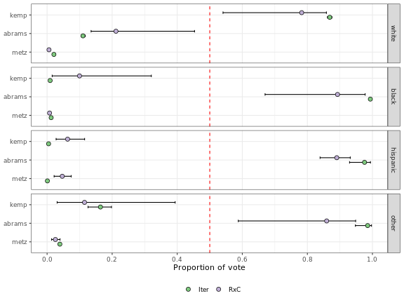
This plot shows the results of both ecological inference methods. The plot presents one panel for each race group. Each panel has a row for each candidate. The x-axis indicates the proportion of the each race group’s vote that is estimated to have gone to each candidate in the election. Lastly, the different colored points represent results from different methods, listed in the legend below the plot.
The top panel, which shows results for white voters, shows that according to both iterative and RxC methods, white voters tended to prefer Brian Kemp over the other candidates in this election. The second panel yields different results for black voters, who show a strong preference for Stacey Abrams over either of the other candidates.
The plotting and summary methods can be used to compare across different methods of ecological inference, or different specifications of the same method.
Summary
This vignette has provided a brief overview of the workflow for using eiCompare to conduct ecological inference. It introduced the following functions:
resolve_missing_vals()dedupe_precincts()stdize_votes_all()plot_bivariate()race_cand_cors()ei_iter()ei_rxc()summary()plot()