eiCompare: Parallel Processing
This vignette aims to highlight the parallel processing capabilities within eiCompare. Functions that include this option are:
-
ei_iter() -
ei_rxc()(only for diagnostic) -
run_geocoder()
Prior to attempting to run these functions in parallel, it is advised you check your computer or server for the following properites:
-
You should have more than 4 physical cores
-
You should have at least 16 GB of RAM
Introduction to parallel processing
Building off of exisiting parallel processing packages such as foreach
and doSNOW, this package includes parallel processing capabiltiies to
speed up ecological inference analyses.
Parallel processing decreases the time needed for your processes by splitting the job amongst your computer’s CPU cores. We recommend 16 GB of RAM so that R can store the data you are currently working on. Furthermore, if you are using multiple cores, the minimum RAM needed is the product of the number of cores you’re using and the size of your data.So if you are working on 4 cores and your dataset is 1 GB, you’ll be using at least 4 GB of RAM.
In order to make this functionality more accessible to users, eiCompare’s functions that include parallel processing include a check for the number of cores you have available to you. If you have less than 4 cores, our functions will not let you proceed with parallelization. Even with exacltly 4 cores, the functions will return a warning that parallelization is not recommended.
There are many resources online if you’d like to learn more about parallelization in general.
Walking through an example: ei_iter()
In this vignette, we’ll be focusing on ei_iter() (the functionalities
and work flow are described in detail in the Ecological Inference
tutorial). We recommend that you review this vignette prior to
attempting parallelization for this function.
The data we’ll be using for this example is from 2014 elections in California, specifically looking at voting results and racial demogrphiacs for Corona by precinct.
head(corona)
#>   precinct totvote pct_husted pct_spiegel  pct_ruth pct_button pct_montanez
#> 1    24000    1626 0.11070111   0.2091021 0.1795818  0.1537515    0.1599016
#> 2    24003    1214 0.10790774   0.2257002 0.1746293  0.1548600    0.1746293
#> 3    24005     732 0.11475410   0.2281421 0.1653005  0.1352459    0.1707650
#> 4    24013    1057 0.08987701   0.2346263 0.1702933  0.1182592    0.2043519
#> 5    24014    1270 0.13149606   0.2299213 0.1834646  0.1259843    0.1629921
#> 6    24015     595 0.09411765   0.2621849 0.1579832  0.1478992    0.1663866
#>     pct_fox  pct_hisp  pct_asian pct_white pct_non_lat
#> 1 0.1869619 0.2483393 0.03730199 0.7143587   0.7516607
#> 2 0.1622735 0.3296460 0.02359882 0.6467552   0.6703540
#> 3 0.1857923 0.3604214 0.05944319 0.5801355   0.6395786
#> 4 0.1825922 0.2364439 0.07377049 0.6897856   0.7635561
#> 5 0.1661417 0.2751764 0.05516357 0.6696600   0.7248236
#> 6 0.1714286 0.2959076 0.14165792 0.5624344   0.7040924
We have a row for every precinct, if we check the dimensions of our dataset you will see that this is 46. We also have 12 variables included in this dataset.
print(dim(corona))
#> [1] 46 12
names(corona)
#>  [1] "precinct"     "totvote"      "pct_husted"   "pct_spiegel"  "pct_ruth"
#>  [6] "pct_button"   "pct_montanez" "pct_fox"      "pct_hisp"     "pct_asian"
#> [11] "pct_white"    "pct_non_lat"
The variables are as follows: - precinct: Precinct ID number
-
totvote: Total number of votes cast -
pct_husted: Percent of voting precinct population who voted for Husted -
pct_spiegel: Percent of voting precinct population who voted for Spiegel -
pct_ruth: Percent of voting precinct population who voted for Ruth -
pct_button: Percent of voting precinct population who voted for Button -
pct_montanez: Percent of voting precinct population who voted for Montanez -
pct_fox: Percent of voting precinct population who voted for Fox -
pct_hisp: Percent of voting precinct population who identify as Hispanic -
pct_asian: Percent of voting precinct population who identify as Asian -
pct_white: Percent of voting precinct population who identify as White -
pct_non_lat: Percent of voting precinct population who identify as Non-Latino
Non-Latino encompasses the Asian and White voting population.
corona$pct_hisp + corona$pct_non_lat == 1
#>  [1] TRUE TRUE TRUE TRUE TRUE TRUE TRUE TRUE TRUE TRUE TRUE TRUE TRUE TRUE TRUE
#> [16] TRUE TRUE TRUE TRUE TRUE TRUE TRUE TRUE TRUE TRUE TRUE TRUE TRUE TRUE TRUE
#> [31] TRUE TRUE TRUE TRUE TRUE TRUE TRUE TRUE TRUE TRUE TRUE TRUE TRUE TRUE TRUE
#> [46] TRUE
So for this analysis there are 6 candidates (Husted, Spiegel, Ruth, Button, and Montanez) and 3 racial groups (Hispanic/Latino, Asian, and White). With that, let’s set up the inputs we need for the function and time it to see how long it takes to complete the iterative ei analysis without parallelization.
cand_cols <- c("pct_husted", "pct_spiegel", "pct_ruth", "pct_button", "pct_montanez", "pct_fox")
race_cols <- c("pct_hisp", "pct_asian", "pct_white")
totals_col <- "totvote"

# Run without parallization
start_time <- Sys.time()
results_test <- ei_iter(corona, cand_cols, race_cols, totals_col)
#> | | | 0% | |======== | 11%
(end_time <- Sys.time() - start_time)
#> Time difference of 1.075621 mins
To run in this parallel, all you need to do is toggle par_compute to
be TRUE.
# Run with paralleization
start_time <- Sys.time()
results_test <- ei_iter(corona, cand_cols, race_cols, totals_col, par_compute = TRUE)
#> | | | 0% | |==== | 6% | |======== | 11% | |============ | 17% | |================ | 22% | |=================== | 28% | |======================= | 33% | |=========================== | 39% | |=============================== | 44% | |=================================== | 50% | |======================================= | 56% | |=========================================== | 61% | |=============================================== | 67% | |=================================================== | 72% | |====================================================== | 78% | |========================================================== | 83% | |============================================================== | 89% | |================================================================== | 94% | |======================================================================| 100%
(end_time <- Sys.time() - start_time)
#> Time difference of 39.73646 secs
This saves us a about a minute for this specific data set. With larger datasets and more candidate and racial demographic comparisons, the process will take longer and parallelization will become more beneficial.
Expectations for parallelization
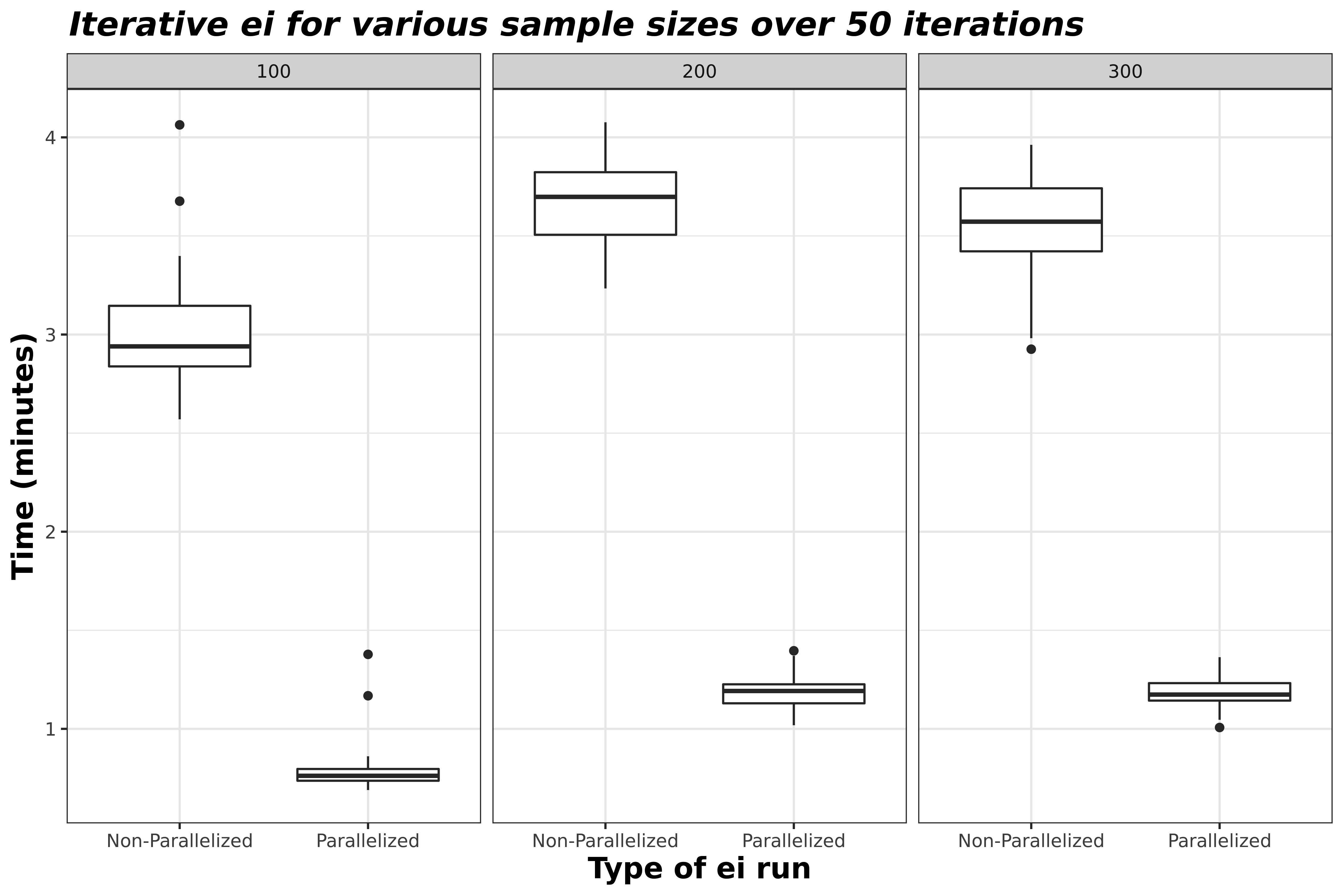
Depending on your dataset, the number of races and candidates you’re analyzung, the amount of RAM you have, and the number of physical and logical cores you have the amount of time it takes to run eiCompare functions will differ. Furthermore, its important to uderstand parallelizing requires overhead time and relationships between sample size and run time are not necessarily linear. In the plot below, you’ll be able to see the average run time of a dataset for a sample of 100, 200, and 300 precincts. It is apparent here that less samples does not equate a shorter run time. Nonetheless, parallelization can save multitudes of the ~4 minutes saved here, especially if you repeat function calls for analyses such as a boostrap.
Summary
eiCompare provides the option to parallelize operations for iterative
ei in ei_iter(), diagnostic tests in ei_rxc(), and geocoding in
run_geocoder(). By setting the parallelization toggle to TRUE, as
well as having the proper set up with more than 4 cores and more than 16
GB of RAM, the user should be able to run these operations multitudes
faster.