eiCompare: Conducting Performance Analyses

This vignette introduces the concept of a performance analysis and demonstrates how eiCompare can be used to conduct one given voter files and districting maps.

What is a performance analysis?

A successful voting rights case may result in a local jurisdiction’s districting map to be thrown out, prompting the need for a new map. Thus, it’s necessary assess whether the new map provides sufficient representation for minority groups. It’s not desirable to simply wait for elections to happen and see what the results might be. Instead, we can look at past elections, and observe how candidates would perform if the proposed map was used at the time of the election. This is the basis of a performance analysis.

Ultimately, we need to assess the demographic breakdown across racial groups for each district in the new map. What data source do we use to calculate the percentage of each racial group? We could use total population or citizen voting age population (CVAP), as provided by the Census Bureau. However, these measures may not be accurate, because they assume that voter turnout is equal across racial groups. This is not always true, especially in cases of racial gerrymandering, where turnout for minority groups may be depressed. Instead, we argue that going to the level of the voter file is necessary, as the voter file actually informs who turned out to vote.

The steps in a performance analysis

To conduct a performance analysis, we need to join the voters in a voter file to the new districts and determine the turnout by race, per district. This includes the following steps:

Geocoding: Geocode latitude and longitude of voters in the file using their address. See the geocoding vignette for more details on this procedure.
Spatial Join: Using the geocoded coordinates, map each voter to the new districts using a spatial join.
Race Estimates: If race is not recorded on the voter file, estimate it using Bayesian Improved Surname Geocoding (BISG) (which itself relies on a spatial join between the voters’ coordinates and Census blocks).
Aggregation: Aggregate the race estimates per district to obtain voter turnout, by race, in each district.

eiCompare provides functions to perform steps 2-4 of the analysis, as well as a function that completes the entire pipeline. Note that Gecoding (step 1) must be performed separately. In the following section, we walk through each of the steps.

Case study: East Ramapo School District

The example we’ll use to demonstrate the performance analysis is East Ramapo School District (ERSD), located in Rockland County of the New York City suburbs. ERSD is highly segregated, with the majority of Black and Hispanic students attending public schools and white students attending private schools. Furthermore, its voting system for the School Board was at-large, where all voters could vote for all seats on the school board. This system favored the white families whose students largely attended private schools, resulting in redistribution of funds that had adverse impacts on public school students.

In May 2020, the at-large voting system was struck down, and a ward system with a new set of districting maps was required. In a ward system, voters elect a representative for their own geographically compact ward. Two maps were proposed: one by the plaintiffs (New York Civil Liberties Union, NYCLU) and the defendants (ERSD). Ideally, the map should allow sufficient representation for the minority aggregate population (in this case, Black and Hispanic/Latino voters).

In this case study, we’ll focus on the defendant map. We’ll demonstrate how a performance analysis reveals that simply using CVAP to assess the minority constituency may overestimate the number of seats won by minority supported candidates.

Ward Map of East Ramapo School District

Let’s take a look at a map proposed by the defendants, ERSD. The district map is composed of nine wards. To assess representation, we could examine the CVAP (the number of people who can vote) by race across the wards. Thus, let’s take a look at the fraction of CVAP voters that are in the minority aggregate, by ward:

# Load the map
data("ersd_maps")

# Plot the map, using a fill that depends on Citizen Voting Age Population (CVAP)
options(repr.plot.width = 7.2, repr.plot.height = 6)
cvap_map <- ggplot() +
  geom_sf(data = ersd_maps, aes(fill = MIN_AGG_FRAC)) +
  geom_sf_label(data = ersd_maps, aes(label = WARD), size = 5) +
  scale_fill_continuous(limits = c(0, 1)) +
  xlab("Latitude") +
  ylab("Longitude") +
  theme_bw(base_size = 10) +
  theme(
    axis.title.x = element_text(size = 15, face = "bold", margin = margin(t = 5)),
    axis.title.y = element_text(size = 15, face = "bold", margin = margin(r = 5)),
    legend.key.width = unit(0.4, "cm"),
    legend.key.height = unit(1, "cm")
  ) +
  guides(fill = guide_legend(
    title = "Fraction\nMinority",
    title.position = "top",
    title.size = 10
  ))
show(cvap_map)

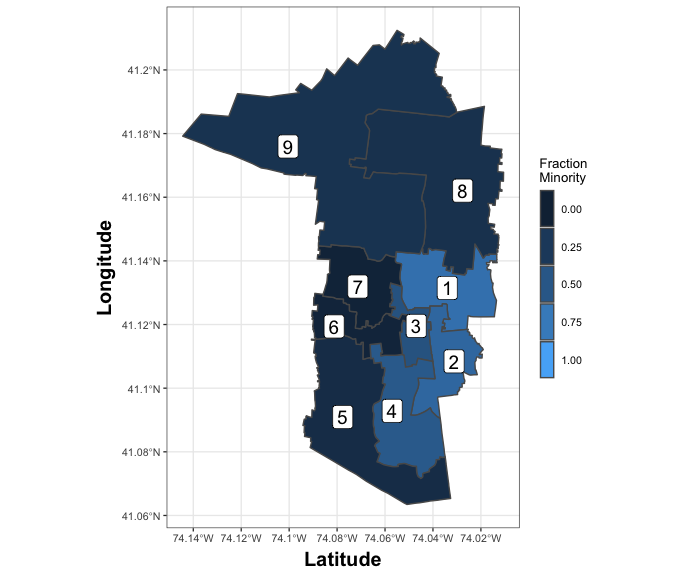
Examining this map reveals that, according to CVAP, four wards (1-4) have potential for minority voters to elect a representative of their choice (they have a plurality or majority). However, due to turnout differences across racial groups, this does not imply that the minority voters would have actually turned out sufficiently enough to elect four representatives. In other words, this map may not have “performed” well enough to guarantee representation, due to turnout.

Toy Voter File

Since the entire pipeline is contained within the function performance_analysis(), we’ll first use a toy voter file to demonstrate the individual steps. This toy voter file already is already “geocoded”, implying that step 1 is complete.

voter_file <- data.frame(
  voter_id = c(1, 2, 3, 4, 5, 5),
  surname = c(
    "ROSENBERG",
    "JACKSON",
    "HERNANDEZ",
    "LEE",
    "SMITH",
    "SMITH"
  ),
  lat = c(41.168, 41.1243, 41.089, 41.14, 41.12, 41.123),
  lon = c(-74.02, -74.039, -74.08, -74.05, -74.045, -74.046)
)

The voter file consists of 5 example voters whose surnames are actually found in the East Ramapo voter file, but locations are randomly assigned. The file depicts the bare necessities for conducting a performance analysis: a voter ID column to identify unique voters, a surname column for identifying race, and latitude/longitude columns for identifying location.

De-duplicating the voter file

Observe that the above voter file contains a duplicate: voter “SMITH” appears twice, with the same voter ID (but different locations). This is a common occurrence in voter files, particularly when voters request a change of address. In these cases, the voter ID remains the same, but both the old and new addresses remain on the voter file for some time. Thus, voter files need to be de-duplicated.

To handle this, eiCompare has a dedupe_voter_file function which will automatically take the most recent entry in the voter file for repeated voter IDs. Voter files are typically sorted by registration date, so de-duplicating automatically takes the latest rows. Let’s apply this function to the toy voter file:

voter_file <- eiCompare::dedupe_voter_file(
  voter_file = voter_file,
  voter_id = "voter_id"
)
print(voter_file)

##   voter_id   surname     lat     lon
## 1        1 ROSENBERG 41.1680 -74.020
## 2        2   JACKSON 41.1243 -74.039
## 3        3 HERNANDEZ 41.0890 -74.080
## 4        4       LEE 41.1400 -74.050
## 6        5     SMITH 41.1230 -74.046

Now, there’s only one row for voter “SMITH” with voter ID “5”. Importantly, it’s the second row in the voter file corresponding to that voter, implying we have the most recent information.

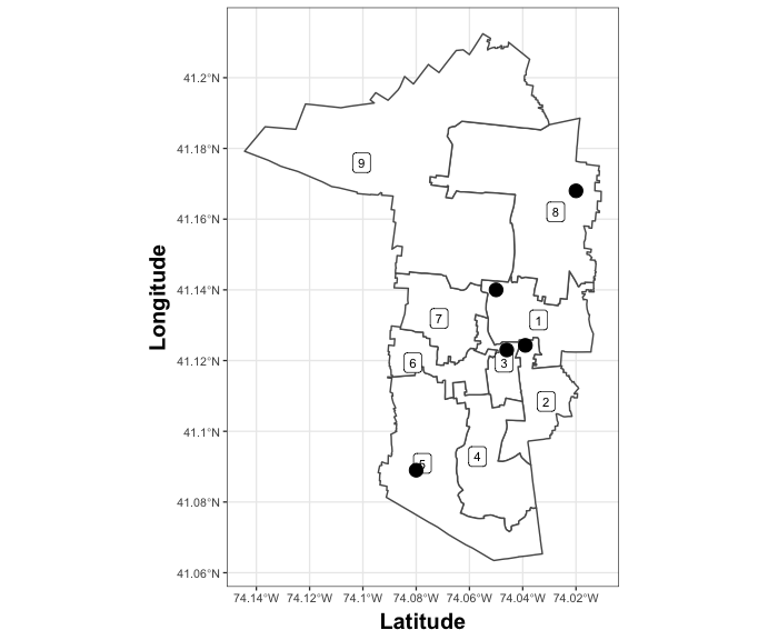
Spatial join between the voter and shape files

Next, we need to identify which wards these voters are located in. Performing this spatial join is abstracted in the merge_voter_file_to_shape() function, which can convert the voter file to a geometry object and join on location. This function, in addition to requiring the voter and shape files, also requires a Coordinates Reference System to use (as a PROJ4 string) as well as the column names for the longitude, latitude, and voter ID (in order to de-duplicate the voter file after the spatial join).

voter_file_w_ward <- eiCompare::merge_voter_file_to_shape(
  voter_file = voter_file,
  shape_file = ersd_maps,
  crs = "+proj=longlat +ellps=GRS80",
  coords = c("lon", "lat"),
  voter_id = "voter_id"
)
print(as.data.frame(voter_file_w_ward)[, c("surname", "WARD")])

##     surname WARD
## 1 ROSENBERG    8
## 2   JACKSON    2
## 3 HERNANDEZ    5
## 4       LEE    1
## 6     SMITH    3

We can double check that the correct wards were identified by plotting the voters on the ward map:

# Plot the map with no fill and voters as points
options(repr.plot.width = 7.2, repr.plot.height = 6)
map <- ggplot() +
  geom_sf(data = ersd_maps, fill = "white") +
  geom_sf_label(data = ersd_maps, aes(label = WARD), size = 3) +
  geom_sf(data = voter_file_w_ward, size = 4, color = "black") +
  xlab("Latitude") +
  ylab("Longitude") +
  theme_bw(base_size = 10) +
  theme(
    axis.title.x = element_text(size = 15, face = "bold", margin = margin(t = 5)),
    axis.title.y = element_text(size = 15, face = "bold", margin = margin(r = 5))
  )
show(map)

This function can also be used to join the voter file to a shapefile of Census blocks, to facilitate predicting race with BISG. Since the Census shape file is too large to include in the package, we’ll simply add the Census information by hand. However, the function would be used in exactly the same way, replacing ersd_maps with the name of the variable containing the Census shape.

voter_file_w_ward$state <- rep("36", 5)
voter_file_w_ward$county <- rep("087", 5)
voter_file_w_ward$tract <- c("010801", "012202", "012501", "011502", "012202")
voter_file_w_ward$block <- c("1016", "3002", "1016", "4001", "2004")

Predicting race using BISG

Since New York state does not report race on the voter file, we need to estimate it using BISG (see the BISG vignette for more details on this approach). Briefly, BISG provides a probabilistic estimate of race by combining knowledge of a voter’s location and surname, both of which are informative of their race. eiCompare has a wrapper function for passing a voter file into the BISG function provided by the WRU package. To use this function, we’ll load some Census data that was extracted using WRU containing information about the racial demographics of Rockland County:

# Load Rockland County Census information
data(rockland_census)

# Apply BISG to the voter file to get race predictions
bisg <- eiCompare::wru_predict_race_wrapper(
  voter_file = as.data.frame(voter_file_w_ward),
  census_data = rockland_census,
  voter_id = "voter_id",
  surname = "surname",
  state = "NY",
  county = "county",
  tract = "tract",
  block = "block",
  census_geo = "block",
  use_surname = TRUE,
  surname_only = FALSE,
  surname_year = 2010,
  use_age = FALSE,
  use_sex = FALSE,
  return_surname_flag = TRUE,
  return_geocode_flag = TRUE,
  verbose = FALSE
)

Let’s take a look at the race probabilities:

print(bisg$bisg[, c(
  "voterid",
  "surname",
  "pred.whi",
  "pred.bla",
  "pred.his",
  "pred.asi"
)])

##   voterid   surname    pred.whi    pred.bla    pred.his     pred.asi
## 1       1 rosenberg 0.861404872 0.025625357 0.011184379 0.0202218400
## 4       2   jackson 0.005119404 0.971940816 0.007282197 0.0007649343
## 5       3 hernandez 0.073473285 0.006983407 0.910532310 0.0051035163
## 2       4       lee 0.228396519 0.602368155 0.013672235 0.1111934217
## 3       5     smith 0.074728196 0.831711494 0.027555904 0.0062517342

These race probabilities have to be merged back into the original voter file, producing a final voter file.

# Merge race information back into voter file
voter_file_final <- dplyr::inner_join(
  x = as.data.frame(voter_file_w_ward),
  y = bisg$bisg[, c(
    "voterid",
    "pred.whi",
    "pred.bla",
    "pred.his",
    "pred.asi",
    "pred.oth"
  )],
  by = setNames("voterid", "voter_id")
)

Lastly, we can get what we set out for: the racial makeup, per ward in the new map. This can be achieved with a simple group-by operation. In the toy voter file, the results won’t make any sense since there’s only five voters. So, let’s look at the final results on an entire voter file.

Running the entire performance analysis

The entire performance analysis pipeline can be performed with the function performance_analysis(). This function handles all of the steps shown above, and outputs the racial turnout per district. Furthermore, it’s equipped with a variety of messaging to provide updates as the analysis is conducted.

To see this function in action, we’ll use it on the East Ramapo voter file. Ordinarily, this voter file would, at the very least, have the same components as the toy voter file (voter id, surname, location). For privacy reasons, we’ve taken the following actions:

Replaced voter ID with new numbers
Replaced the surname with a “similar” surname, in terms of probability across racial groups (ultimately having little impact on the performance analysis). Surnames not found in the Census database are replaced with the string “NOTINCENSUS”, with the same effect of probabilities being imputed according to the Census specification.
Spatially joined the location into the Census block and ward in an effort to not include latitude and longitude.

Let’s take a look at the voter file:

# Load Ramapo 2018 voter file
data("ramapo2018")
print(head(ramapo2018, 10))

##    voter_id     last_name ward state county  tract block
## 1         1       HINKSON    9    36    087 011501  3012
## 2         2    BLUMENTHAL    9    36    087 011501  2014
## 3         3    BLUMENTHAL    9    36    087 011501  2014
## 4         4    PATTENAUDE    9    36    087 011501  4008
## 5         5    PATTENAUDE    9    36    087 011501  4008
## 6         6       RODBERG    9    36    087 011501  2009
## 7         7 NOCENSUSMATCH    9    36    087 011501  3001
## 8         8 NOCENSUSMATCH    9    36    087 011501  3001
## 9         9          COLE    9    36    087 011501  3009
## 10       10          COLE    9    36    087 011501  3009

We can see that the voters already have the FIPS codes and wards identified. Furthermore, some surnames are “NOCENSUSMATCH”, which indicate that these voters’ surnames weren’t found in the Census surname database.

The performance analysis function can handle a variety of scenarios, provided a voter file. For example, if a voter file needs to be spatially joined with the Census shapefile or ward shapefile, it can perform those joins. If not, it will use information already stored in the voter file. To clarify the particular scenario, we need to specify the correct parameters in the function signature. In the Ramapo 2018 case, we specify join_census_shape = FALSE and join_district_shape = FALSE, since the voter file already has this information. This implies that we don’t need to provide shapefiles.

Let’s run the performance analysis:

# Load Ramapo 2018 voter file
data("ramapo2018")

# Run Performance Analysis
results <- eiCompare::performance_analysis(
  voter_file = ramapo2018,
  census_data = rockland_census,
  join_census_shape = FALSE,
  join_district_shape = FALSE,
  state = "NY",
  voter_id = "voter_id",
  surname = "last_name",
  district = "ward",
  census_state_col = "state",
  census_county_col = "county",
  census_tract_col = "tract",
  census_block_col = "block",
  crs = "+proj=longlat +ellps=GRS80",
  coords = c("lon", "lat"),
  census_geo = "block",
  use_surname = TRUE,
  surname_only = FALSE,
  surname_year = 2010,
  use_age = FALSE,
  use_sex = FALSE,
  normalize = TRUE,
  verbose = TRUE
)

## Voter file has 9401 rows.
## Beginning functionality analysis...

## De-duplicating removed 0 voters. Voter file now has 9401 rows.
## Merging voter file with census shape files.

## Voter file already matched to Census shapefile.

## Voter file already matched to district shape.

## Matching surnames.

## Performing BISG to obtain race probabilities.

## Some voters failed geocode matching. Matching at a higher level.

## BISG complete.

## BISG didn't match 1126 surnames.
## BISG didn't match 75 geocodes.

## Performance analysis complete.

Notice that the function outputted messages during the process, since we specified verbose = TRUE.

With the performance analysis complete, let’s compare the predicted turnout of the minority aggregate to the CVAP fraction:

options(repr.plot.width = 5, repr.plot.height = 5)

# Get minority aggregate turnout
performance <- results$results
ersd_maps$MIN_AGG_FRAC_TURNOUT <- performance$black + performance$hispanic

# Run performance analysis
performance_comparison <- ggplot(ersd_maps, aes(x = MIN_AGG_FRAC, y = MIN_AGG_FRAC_TURNOUT)) +
  geom_point(size = 3) +
  geom_abline(intercept = 0, slope = 1) +
  geom_hline(
    yintercept = 0.5,
    linetype = "dashed",
    color = "red",
    size = 1
  ) +
  geom_text(aes(label = WARD), hjust = 0.45, vjust = 1.75) +
  geom_vline(
    xintercept = 0.5,
    linetype = "dotted",
    color = "purple",
    size = 1
  ) +
  xlim(0, 1) +
  ylim(0, 1) +
  ggtitle("Minority Aggregate Voter Share") +
  xlab("CVAP Prediction") +
  ylab("Performance Analysis Prediction") +
  coord_fixed() +
  theme_bw() +
  theme(
    plot.title = element_text(hjust = 0.5, size = 15, face = "bold"),
    axis.text.x = element_text(size = 12),
    axis.title.x = element_text(size = 15, face = "bold"),
    axis.text.y = element_text(size = 12),
    axis.title.y = element_text(size = 15, face = "bold")
  )
show(performance_comparison)

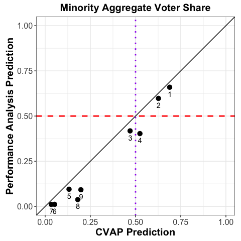
We observe that the turnout is below the CVAP predictions (identity line). Furthermore, using turnout reveals that Districts 3 and 4, despite having a large enough CVAP population for minority seats (or close to it: dotted purple line), would have much lower minority vote given turnout (dashed red line). Thus, the performance analysis demonstrates that using CVAP would exaggerate the number of seats awarded to minority candidates on the school board. In reality, only two seats would likely be awarded to minority-favored candidates, implying the need for a new map.

Voting Rights